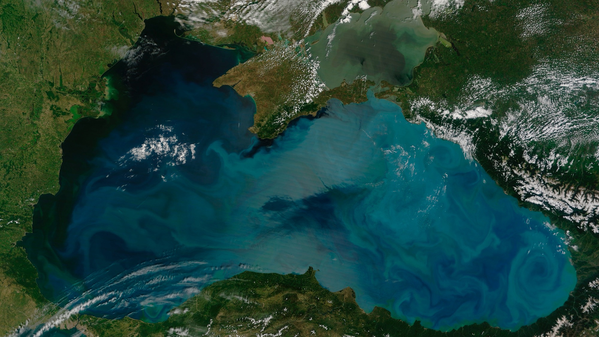
Marketing Scoops: The Tiny Ocean Organisms That Could Help The Climate In a Big Way

Stocktrek Images / Getty Images

Some of the littlest organisms in the ocean wield incredible influence, both on their ecosystems and on the planet. Like plants do on land, phytoplankton absorb sunlight and carbon dioxide and expel oxygen. They process so much of those two gases, in fact, that they’re responsible for half of the carbon sequestered by photosynthesis worldwide and half of the oxygen in the atmosphere…….Continue reading….

By: Matt Simon / Grist

Source: Popular Science

Critics:

The initial concept of visualizing historical temperature data has been extended to involve animation, to visualize sea level rise and predictive climate data, and to visually juxtapose temperature trends with other data such as atmospheric CO₂ concentration, global glacier retreat, precipitation, progression of ocean depths, aviation emission’s percentage contribution to global warming, biodiversity loss, soil moisture deviations, and fine particulate matter concentrations.

In less technical contexts, the graphics have been embraced by climate activists, used as cover images of books and magazines, used in fashion design, projected onto natural landmarks, and used on athletic team uniforms, music festival stages, and public infrastructure. Warming stripe graphics are defined with various parameters, including:

source of dataset (meteorological organization)
geographical scope of measurement (global, country, state, etc.)
time period (year range, for horizontal “axis”)
temperature range (range of anomaly (deviation) about a reference or baseline temperature)
colour palette (usually, shades of blue and red),
colour scale (assignment of colours to represent respective ranges of temperature anomaly),
temperature boundaries (temperature above which a stripe is red and below which is blue, usually determined by an average annual temperature over a “reference period” or “baseline” of usually 30 years).

Hawkins’ original graphics use the eight most saturated blues and reds from the ColorBrewer 9-class single hue palettes, which optimize colour palettes for maps and are noted for their colourblind-friendliness. Hawkins said the specific colour choice was an aesthetic decision (“I think they look just right”), also selecting baseline periods to ensure equally dark shades of blue and red for aesthetic balance.

Hawkins chose the 1971-2000 average as a boundary between reds and blues because the average global temperature in that reference period represented the mid-point in the warming to date. A Republik analysis said that “this graphic explains everything in the blink of an eye”, attributing its effect mainly to the chosen colors, which “have a magical effect on our brain, (letting) us recognize connections before we have even actively thought about them”.

The analysis concluded that colors other than blue and red “don’t convey the same urgency as (Hawkins’) original graphic, in which the colors were used in the classic way: blue=cold, red=warm.” ShowYourStripes.info cites dataset sources Berkeley Earth, NOAA, UK Met Office, MeteoSwiss, DWD (Germany), specifically explaining that the data for most countries comes from the Berkeley Earth temperature dataset, except that for the US, UK, Switzerland & Germany the data comes from respective national meteorological agencies.

For statistical and geographic reasons, it is expected that graphics for small areas will show more year-to-year variation than those for large regions. Year-to-year changes reflected in graphics for localities result from weather variability, whereas global warming over centuries reflects climate change. The NOAA website warns that the graphics “shouldn’t be used to compare the rate of change at one location to another”, explaining that “the highest and lowest values on the colour scale may be different at different locations”.

Further, a certain colour in one graphic will not necessarily correspond to the same temperature in other graphics. A climate change denier generated a warming stripes graphic that misleadingly affixed Northern Hemisphere readings over one period to global readings over another period, and omitted readings for the most recent thirteen years, with some of the data being 29-year-smoothed—to give the false impression that recent warming is routine.

For each country-level graphic (Hawkins, June 2019), the average temperature in the 1971–2000 reference period is set as the boundary between blue (cooler) and red (warmer) colours, the colour scale varying +/- 2.6 standard deviations of the annual average temperatures between 1901 and 2000. Hawkins noted in 2019 that the graphic for the Arctic “broke the colour scale” since it is warming more than twice as fast as the global average,and reported that the 2023 global average was so extreme that a new, darker shade of red was required.

For statistical and geographic reasons, it is expected that graphics for small areas will show more year-to-year variation than those for large regions. Year-to-year changes reflected in graphics for localities result from weather variability, whereas global warming over centuries reflects climate change. Some warned that warming stripes of individual countries or states, taken out of context, could advance the idea that global temperatures are not rising, though research meteorologist J. Marshall Shepherd said that “geographic variations in the graphics offer an outstanding science communication opportunity”.

Fill a gap and enable communication with minimal scientific knowledge required to understand their meaning”. J. Marshall Shepherd, former president of the American Meteorological Society, lauded Hawkins’ approach, writing that “it is important not to miss the bigger picture. Science communication to the public has to be different” and commending Hawkins for his “innovative” approach and “outstanding science communication” effort.

This Striking Climate Change Visualization Is Now Customizable for Any Place on Earth”.

Show your stripes: These striking graphics that portray a warming climate are available for countries and regions”.

Climate stripes” graphics show U.S. trends by state and county”.

Visualisierungswettbewerb “Vis for Future” – das sind die Gewinner*innen”

Ed Hawkins’ warming stripes add colour to climate communication”.

This Climate Visualization Belongs in a Damn Museum”.

This Has Got to Be One of The Most Beautiful And Powerful Climate Change Visuals We’ve Ever Seen”.

Why this climate change data is on flip-flops, leggings, and cars / Warming stripes keep showing up on clothes and crafts”.

One of the most striking trends – over a century of global-average sea level change”.

Sea-Level Rise from the Late 19th to the Early 21st Century”

New Climate Change Visualization Presents Two Stark Choices For Our Future”.

Climate Change Visualizations”.